Standardizing a random vector and applications

Motivation

In probability and statistics, standardization is a process that scales and centers variables. For a scalar random variable $X$, its standardization is the variable $Z$ defined by

Standardization allows for easier comparison and analysis of different variables, providing a common ground for meaningful interpretations. A good example of this is the use of standardized coefficients in regression.

If $X$ is instead a random vector, the above formula falls short since $\operatorname{Var}(X)$ is a covariance matrix. In this short exposition, the above formula is generalized to the vector (a.k.a. multivariate) setting.

As an application, we consider a well-known recipe for sampling from multivariate random normal distributions using a standard random normal sampler.

Prerequisites

• Independence
• Random vector
• Covariance matrix
• Positive definite matrix
• Cholesky factorization
• Multivariate normal distribution

Standardizing a random vector

Standardization in multiple dimensions is an immediate consequence of the following result:

Proposition (First and Second Moments of Affine Transform). Let $U$ and $V$ be random vectors, $A$ be a (deterministic) matrix and $b$ be a (deterministic) vector such that

Then,

You can prove the above by direct computation, using linearity of expectation and the identity $\operatorname{Var}(Y) = \mathbb{E}[YY^\intercal] - \mathbb{E}Y\mathbb{E}Y^\intercal$.

Corollary (Standardization). Let $\mu$ be a vector and $\Sigma$ be a positive definite matrix so that it admits a Cholesky factorization $LL^\intercal = \Sigma$. Let $X$ and $Z$ be random vectors satisfying

Then, $X$ has mean $\mu$ and covariance matrix $\Sigma$ if and only if $Z$ has mean $\mathbf{0}$ and covariance matrix $I$.

Note that in the above, $L$ generalizes $\sqrt{\operatorname{Var}(X)}$ from the scalar case.

Bivariate case

It is useful, for the sake of reference, to derive closed forms for the Cholesky factorization in the $d = 2$ case. In this case, the covariance matrix takes the form

It is easy to verify (by matrix multiplication) that the Cholesky factorization is given by

Its inverse is

Sampling a multivariate random normal distribution

A multivariate random normal variable is defined as any random vector $X$ which can be written in the form

where $Z$ is a random vector whose coordinates are independent standard normal variables. From our results above, we know that $X$ has mean $\mu$ and covariance $\Sigma = LL^\intercal$.

Remark. This only one of many equivalent ways to define a multivariate random normal variable.

This gives us a recipe for simulating draws from an arbitrary multivariate random normal distribution given only a standard random normal sampler such as np.random.randn():

def sample_multivariate_normal(
    mean: np.ndarray,
    covariance: np.ndarray,
    n_samples: int = 1,
) -> np.ndarray:
    """Samples a multivariate random normal distribution.
    
    Parameters
    ----------
    mean
        ``(d, )`` shaped mean
    covariance
        Positive definite ``(d, d)`` shaped covariance matrix
    n_samples
        Number of samples

    Returns
    -------
    ``(n_samples, d)`` shaped array where each row corresponds to a single draw from a multivariate normal.
    """
    chol = np.linalg.cholesky(covariance)
    rand = np.random.randn(mean.shape[0], n_samples)
    return (chol @ rand).T + mean

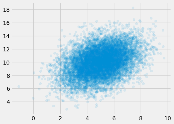
We can verify this is working as desired with a small test and visualization:

mean       = np.array([5., 10.])
covariance = np.array([[2., 1.],
                       [1., 4.]])

samples = sample_multivariate_normal(mean=mean,
                                     covariance=covariance,
                                     n_samples=10_000)

x, y = samples.T
plt.scatter(x, y, alpha=0.1)

empirical_covariance = np.cov(samples, rowvar=False)

print(f"""
Empirical covariance:
{empirical_covariance}

True covariance:
{covariance}
""")

Empirical covariance:
[[1.96748266 1.02186592]
 [1.02186592 3.98317796]]

True covariance:
[[2. 1.]
 [1. 4.]]