Maximum likelihood estimation of geometric Brownian motion parameters

Motivation

Given an asset’s historical prices over some time horizon (e.g., the price of APPL on each trading day of 2019), it is often of practical importance to fit a distribution to those prices.

One choice of parametric model for stock prices is geometric Brownian motion (GBM). This note derives maximum likelihood estimators for the parameters of a GBM.

A word of caution: a GBM is generally unsuitable for long periods. Other choices of models include a GBM with nonconstant drift and volatility, stochastic volatility models, a jump-diffusion to capture large price movements, or a non-parametric model altogether. Regardless of what choice is made, it is prudent to perform a goodness of fit test (outside of the scope of this note) a posteriori.

Geometric Brownian motion

Consider an asset $S$ which follows geometric Brownian motion (GBM) with constant drift $\mu$ and volatility $\sigma$:

\[dS_{t}=\mu S_{t}dt+\sigma S_{t}dW_{t}.\]

By Ito’s lemma, $X_{t}=\log S_{t}$ satisfies

\[dX_{t}=\left(\mu-\frac{1}{2}\sigma^{2}\right)dt+\sigma dW_{t}.\]

Suppose the asset’s prices are observed at the sequence of (increasing) times $t_{0},t_{1},\ldots,t_{N}$. By the previous paragraph,

\[\Delta X_{n}=\left(\mu-\frac{1}{2}\sigma^{2}\right)\Delta t_{n}+\sigma\Delta W_{n}\]

where $\Delta X_{n}=X_{t_{n}}-X_{t_{n-1}}$, $\Delta t_{n}=t_{n}-t_{n-1}$, and $\Delta W_{n}=W_{t_{n}}-W_{t_{n-1}}$. In particular, $\Delta X_{n}$ is normal with mean $(\mu-\frac{1}{2}\sigma^{2})\Delta t_{n}$ and variance $\sigma^{2}\Delta t_{n}$.

Maximum likelihood estimation

Let $\delta X=X_{t_{N}}-X_{t_{0}}$ and $\delta t=t_{N}-t_{0}$ for brevity. The main result is summarized below.

Proposition. The maximum likelihood estimators (MLE) of the drift and volatility are

\[\hat{\mu} =\frac{\delta X}{\delta t}+\frac{1}{2}\hat{\sigma}^{2}\]

and

\[\hat{\sigma}^{2} =-\frac{1}{N}\frac{\left(\delta X\right)^{2}}{\delta t}+\frac{1}{N}\sum_{n=1}^{N}\frac{\Delta X_{n}^{2}}{\Delta t_{n}}.\]

In the case of evenly spaced time intervals ($\Delta t_{n} = \delta t / N$), $\hat{\sigma}^{2}$ simplifies to

\[\hat{\sigma}^{2}=-\frac{1}{N}\frac{\left(\delta X\right)^{2}}{\delta t}+\frac{1}{\delta t}\sum_{n=1}^{N}\Delta X_{n}^{2}.\]

The derivation of the proposition is given in the final section of this note.

Remark. If the exact value of the volatility is known a priori, the MLE $\hat{\mu}$ above can still be used by replacing $\hat{\sigma}$ with $\sigma$. On the other hand, if the exact value of the drift is known a priori, the expression for $\hat{\sigma}$ above is not an MLE. The appropriate expression in this case is given in the final section of this note.

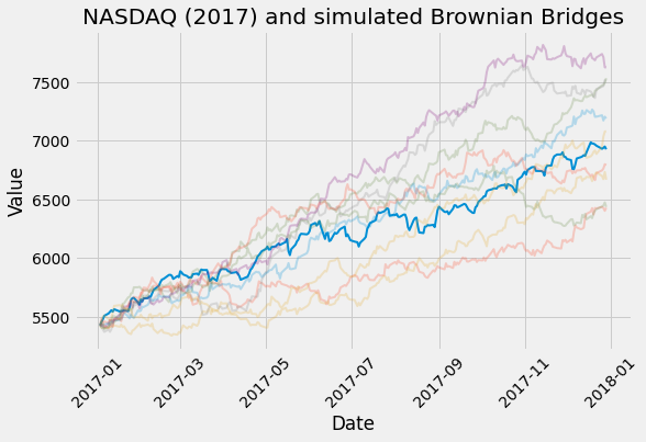
Estimating NASDAQ drift and volatility in 2017

import numpy as np
import yfinance as yf

ticker = yf.Ticker("^IXIC")  # NASDAQ
df = ticker.history(start="2017-01-01", end="2017-12-31")

price = (df.Open + df.Close) / 2.0
price = price.values

log_price = np.log(price)  # X
delta = log_price[1:] - log_price[:-1]  # ΔX
n_samples = delta.size  # N
n_years = 1.0  # δt
total_change = log_price[-1] - log_price[0]  # δX

vol2 = (-(total_change**2) / n_samples + np.sum(delta**2)) / n_years
# Equivalent but slower: `vol2 = np.var(delta) * delta.size / n_years`
vol = np.sqrt(vol2)

drift = total_change / n_years + 0.5 * vol2

print("drift: {0:06.3f}%".format(drift * 100))
print("vol:   {0:06.3f}%".format(vol * 100))

drift: 24.696%
vol:   07.530%

The true value of the NASDAQ along with 9 GBM simulations using the drift and volatility parameters above are shown below.

png

Derivation

The MLE are obtained by maximizing the log-likelihood

\[\ell=\sum_{n=1}^{N}\log f_{n}(\Delta X_{n})\]

where $f_{n}$ is the density of $\Delta X_{n}$. In particular,

\[\log f_{n}(\Delta X_{n})=-\ln(\sigma)-\frac{\left(\Delta X_{n}-\left(\mu-\frac{1}{2}\sigma^{2}\right)\Delta t_{n}\right)^{2}}{2\sigma^{2}\Delta t_{n}}+\text{const.}\]

Some calculus reveals

\[\frac{\partial\log f_{n}(\Delta X_{n})}{\partial\mu}=\frac{\Delta X_{n}-\left(\mu-\frac{1}{2}\sigma^{2}\right)\Delta t_{n}}{\sigma^{2}}.\]

Therefore,

\[\frac{\partial\ell}{\partial\mu}=\frac{\delta X-\left(\mu-\frac{1}{2}\sigma^{2}\right)\delta t}{\sigma^{2}}.\]

Setting this to zero and solving for $\mu$ yields the MLE

\[\hat{\mu}=\frac{\delta X}{\delta t}+\frac{1}{2}\sigma^{2}.\]

Similarly,

\[\frac{\partial\log f_{n}(\Delta X_{n})}{\partial\sigma}=\frac{\left(\mu^{2}-\frac{1}{4}\sigma^{4}\right)\Delta t_{n}-\sigma^{2}-2\mu\Delta X_{n}+\Delta X_{n}^{2}\Delta t_{n}^{-1}}{\sigma^{3}}.\]

Therefore,

\[\frac{\partial\ell}{\partial\sigma}=\frac{\left(\mu^{2}-\frac{1}{4}\sigma^{4}\right)\delta t-N\sigma^{2}-2\mu\delta X+\sum_{n}\Delta X_{n}^{2}\Delta t_{n}^{-1}}{\sigma^{3}}.\]

Setting the above to zero and solving for $\hat{\sigma}$ yields the MLE

\[\hat{\sigma}^{2}=2\frac{\sqrt{\delta t\left(\mu^{2}\delta t-2\mu\delta X+\sum_{n}\Delta X_{n}^{2}\Delta t_{n}^{-1}\right)+N^{2}}-N}{\delta t}.\]