Hypothesis testing for mathematicians

Most introductions to hypothesis testing are targeted at non-mathematicians. This short post aims to be a precise introduction to the subject for mathematicians.

Remark. While the presentation may differ, some of the notation in this article is from L. Wasserman’s All of Statistics: a Concise Course in Statistical Inference.

Consider a parametric model with parameter set $\Theta$. The model generates realizations $X_1, \ldots, X_n$.

Example (Coin Flip). We are given a coin. The coin has probability $\theta$ in $\Theta \equiv [0, 1]$ of showing heads. We flip the coin $n$ times and record $X_i = 1$ if the $i$-th flip is heads and $0$ otherwise.

Throughout this article, we use the above coin flip model to illustrate the ideas.

In hypothesis testing, we start with a hypothesis (also called the null hypothesis). Specifying a null hypothesis is equivalent to picking some nonempty subset $\Theta_0$ of the parameter set $\Theta$. Precisely, the null hypothesis is the assumption that realizations are being generated by the model parameterized by some $\theta$ in $\Theta_0$.

Example (Coin Flip). Our hypothesis is $\Theta_0 \equiv { 1 / 2 }$. That is, we hypothesize that the coin is fair.

For brevity, let $X \equiv (X_1, \ldots, X_n)$. To specify when the null hypothesis is rejected, we define a rejection function $R$ such that $R(X)$ is an indicator random variable whose unit value corresponds to rejection.

Example (Coin Flip). Let

\[R(x_1, \ldots, x_n) = \left[ \left| \frac{x_1 + \cdots + x_n}{n} - \frac{1}{2} \right| \geq \epsilon \right]\]

where $[\cdot]$ is the Iverson bracket. This corresponds to rejecting the null hypothesis whenever we see “significantly” more heads than tails (or vice versa). Our notion of significance is controlled by $\epsilon$.

Note that nothing stops us from making a bad test. For example, taking $\epsilon = 0$ in the above example yields a test that always rejects. Conversely, taking $\epsilon > 1/2$ yields a test that never rejects.

Definition (Power). The power

\[\operatorname{Power}(\theta, R) \equiv \mathbb{P}_\theta \{ R(X) = 1 \}\]

gives the probability of rejection assuming that the true model parameter is $\theta$.

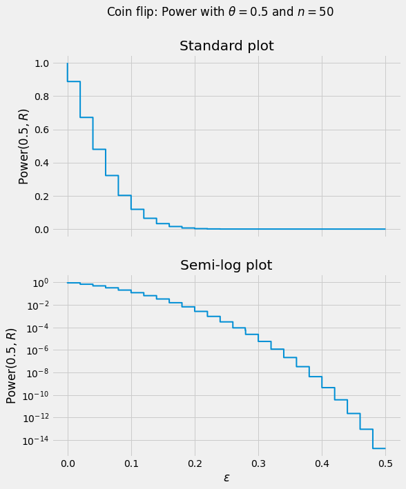
Example (Coin Flip). Let $F_\theta$ denote the CDF of a binomial distribution with $n$ trials and success probability $\theta$. Let $S \equiv X_1 + \cdots + X_n$. Then, assuming $\epsilon$ is positive,

\[\operatorname{Power}(\theta,R) = 1 - \mathbb{P}_{\theta}\{\left|S/n-1/2\right| < \epsilon\} = 1 - \mathbb{P}_{\theta}\{n/2-\epsilon n < S < n/2+\epsilon n\} = 1 - F_\theta(\left(n/2+\epsilon n\right)-) + F_\theta(n/2-\epsilon n)\]

where $F(x-) = \lim_{y \uparrow x} F(y)$ is a left-hand limit.

Definition (Size). The size of a test

\[\operatorname{Size}(R) \equiv \sup_{\theta \in \Theta_0} \operatorname{Power}(\theta, R)\]

gives, assuming that the null hypothesis is true, the “worst-case” probability of rejection.

Rejecting the null hypothesis errenously is called a type I error (see the table below). The size puts an upper bound on making a type I error.

	Retain Null	Reject Null
Null Hypothesis is True	No error	Type I error
Null Hypothesis is False	Type II error	No error

Example (Coin Flip). Since $\Theta_0 = { 1 / 2 }$ is a singleton, $\operatorname{Size}(R) = \operatorname{Power}(1/2, R)$.

Definition (p-value). Let $(R_\alpha)_\alpha$ be a collection of rejection functions. Define

\[\operatorname{p-value} \equiv \inf \left\{ \operatorname{Size}(R_\alpha) \colon R_\alpha(X) = 1 \right\}\]

as the smallest size for which the null-hypothesis is rejected.

Unlike the size, the p-value is itself a random variable. The smaller the p-value, the more confident we can be that a rejection is justified. A common threshold for rejection is a p-value smaller than 0.01. A rejection in this case can be understood as being at least 99% certain the rejection was not done erroneously.

Theorem 1. Suppose we have a collection of rejection functions $(R_{\alpha})_{\alpha}$ of the form

\[R_{\alpha}(x_1, \ldots, x_n) = [f(x_1, \ldots, x_n) \geq c_{\alpha}]\]

where $f$ does not vary with $\alpha$. Suppose also that for each point $y$ in the range of $f$, there exists $\alpha$ such that $c_{\alpha} = y$. Then,

\[\operatorname{p-value}(\omega) \equiv \sup_{\theta \in \Theta_0} \mathbb{P}_{\theta} \{ f(X) \geq f(X(\omega)) \}.\]

In other words, the p-value (under the setting of Theorem 1) is the worst-case probability of sampling $f(X)$ larger than what was observed, $f(X(\omega))$. Note that in the above, we have used $\omega$ to distinguish between the actual random variable $X$ and $X(\omega)$, the observation.

Proof. Recall that the p-value is an infimum among sizes of tests that reject the observed data. The infimum is achieved at $c_\alpha = f(X(\omega))$. This is because a larger value of $c_\alpha$ yields a test that accepts while a smaller value yields a test that rejects at least as many outcomes, thereby potentially having larger size. The size under the choice of $c_\alpha = f(X(\omega))$ is exactly the expression for the p-value given above. $\square$

Example (Coin Flip). We flip the coin $n$ times and observe $S(\omega)$ heads. By Theorem 1,

\[\operatorname{p-value}(\omega) = \mathbb{P}_{1/2} \left\{ \left|S/n - 1/2\right| \geq \left|S(\omega)/n - 1/2\right| \right\}.\]

Let

\[K(\omega) = |S(\omega) - n/2|.\]

Then,

\[\operatorname{p-value}(\omega) = 1 - \mathbb{P}_{1/2} \left\{ n/2 - K(\omega) < S < n/2 + K(\omega) \right\} = 1 - F_{1/2}(\left(n/2 + K(\omega)\right)-) + F_{1/2}(n/2 - K(\omega)).\]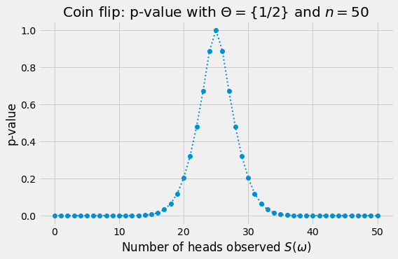

Theorem 2. Suppose the setting of Theorem 1 and that, in addition, $\Theta_0 = {\theta_0}$ is a singleton and $f(X)$ has a continuous and strictly increasing CDF under $\theta_0$. Then, the p-value has a uniform distribution on $[0,1]$ under $\theta_0$.

In other words, if the null hypothesis is true, the p-value (under the setting of Theorem 2) is uniformly distributed on $[0, 1]$.

Proof. Denote by $G$ the CDF of $f(X)$ under $\theta_0$. By Theorem 1,

\[\operatorname{p-value}(\omega) = 1 - G[f(X(\omega))].\]

Then (omitting the subscript $\theta_0$ for brevity),

\[\mathbb{P} \{ \omega \colon \operatorname{p-value}(\omega) \leq u \} = 1 - \mathbb{P} \{ \omega \colon G[f(X(\omega))] \leq 1 - u \} = 1 - \mathbb{P} \{ \omega \colon f(X(\omega)) \leq G^{-1}(1 - u) \} = 1 - G(G^{-1}(1 - u)) = u. \square\]